Add disorder by Kwant

X.-Z. CHEN, 23/05/2024, EIT, Ningbo

Disorder

Disorder enters the Hamiltonian as a disorder potential $V_{dis}$. There are various models for such potentials. A very commonly used model is to add a random on-site potential to the tight-binding model:

$$V_{dis} = \sum_{i} U_i |x_i\rangle \langle x_i |$$

where $U_i$ are choosen randomly from a uniform distribution $[-U_0/2,U_0/2]$.

It is worth nothing that the disorder strength $U_0$ by itself does not mean much. Instead one must quantify the disorder strength by an physical quantity. For disorder this is the mean field path. From Fermi’s golden rule, one can compute that for this model

$$l_{\rm{mfp}}=48a\frac{\sqrt{E/t}}{(U_0/t)^2}$$

where $a$ is again the lattice constant, $t$ the hopping energy on the square lattice.

Magnetic/Nonmagnetic short/long-range disorder

Refs: PRL 125 157402 (2020)

For valley-related transport, the influence of the short- and long-range disorder is usually significatly different since the former (later) induces (excludes) intervalley scattering, which has been well explored in graphene [RMP 83 407 (2011)]. The short (long)-range disorder is characterized by the smaller (larger) disorder correlation length $\lambda$, compared to the lattice spaceing, $a$ [RMP 83 407 (2011), EPL 79 57003 (2007)]. Their crossover can be well described by a Gaussian correlated disorder potential of

$$\eta(r)=\omega e^{-r^2/\lambda^2},$$

where $\omega$ parametrizes the disorder strength. Specifically, for a short-range disorder, usually induced by the point defects [RMP 83 407 (2011)], its disorder potential localizes in the atomic range ($\lambda<0$) 79 83 407 57003 and the induced intervalley scattering enables strong backscattering, eventually turning conducting system into an anderson insulator. such a short-range disorder is also called disorder, when $\lambda\rightarrow 0$ [[rmp (2011)](), [epl (2007)]()]. in contrast, for long-range often arising from charged impurities or ripples (2011)]()], its potential smooth on scale of lattice spacing ($\lambda> a$) and there is very little intervalley scattering. As a result, the back scattering is suppressed and the system remains highly conductive [RMP 83 407 (2011), EPL 79 57003 (2007)].

To explore the influence of the short-range and long-range disorder of the system, we can add a nonmagnetic disorder term

$$H_{ND} = \sum_{i} c_i^{\dagger}\eta_i \begin{pmatrix} 1 & 1\\ 1 & 1\\ \end{pmatrix} \otimes \sigma_0 c_i.$$

Here, we rewrite $\eta(r)$ in a discrete model as

$$\eta_i = \sum_{j=1}^{N_p} \omega_j e^{-|r_{ij}/\lambda|^2},$$

where $|r_{ij}|$ is the distance between site $i$ and $j$, $N_p$ is the total number of the scattering centers, which, dividing the total number ($N$) of the lattice sites, gives the disorder probability, $P=N_p/N$.

To explore the crossover of short-range and long-range disorder, we induce the magnetic short/long-range disorder to break the TRS and thus validating the intervalley scattering. When TRS is broken, the QSVHK degrades into the QVHK, and then it is expected to be robust against the magnetic long-range disorder, but can be intervalley-scattered by the magnetic short-range disorder. The magnetic disorder is induced by adding an in-plane magnetic exchange field

$$H_{MD}=\sum_{i} c_{i}^{\dagger} \eta_i \begin{pmatrix} 1 & 1\\ 1 & 1\\ \end{pmatrix}\otimes \sigma_x c_i$$

Numerical

example1: Add disorder through homemade method

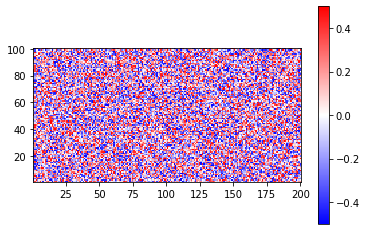
def random_potential(site,w):
        pot = np.random.random()
        pot_w = w*(2*pot - 1)
    return pot_w

example2: Add short-range disorder through kwant

def random_potential(site):
    return w*(2*uniform(repr([site]),salt)-1)

Here, note that uniform(input,salt), the input and salt should both be a string, the detailed use method is that input should vary by sites, and salt should be a series vary index.

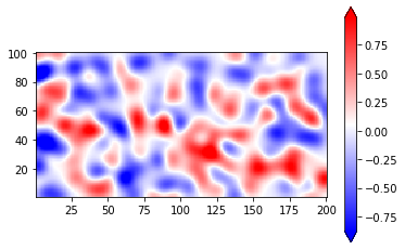
example3: Add long-range disorder through kwant

def pot(site,xi,yi):
    x,y = site.pos
    return U0*np.exp(-((x-xi)**2/(2*sigmax**2)+(y-yi)**2/(2*sigmay**2)))

def random_potential(site):
    pot_val = pot(site,xis[0],yis[0])
    for i,xi in enumerate(xis[1:len(xis)]):
        if i < int(len(xis)/2):
            pot_temp = pot(site,xi,yis[i])
        else:
            pot_temp = -pot(site,xi,yis[i])
        pot_val = pot_val + pot_temp
    return pot_val